[Pytorch] RNN(Recurrent Neural Network)

딥러닝

[Pytorch] RNN(Recurrent Neural Network)

Woohh 2024. 10. 18. 02:13

RNN(Recurrent Neural Network) with Pytorch

Pytorch를 통해 기존에 작성한 RNN 모델을 실제로 구현해볼 것이다.

RNN 모델 학습에 필요한 데이터는 코드를 통해 직접 생성할 것이다.

Import

우선 필요한 것들을 Import 해준다.

import torch
import torch.nn as nn
import torch.optim as optim
import torch.nn.functional as F

import numpy as np

import matplotlib.pyplot as plt

Dataset

수열의 형태로 만들 것이며, 수열 내의 각 원소의 값은 0~9 중에서 랜덤하게 설정한다.

이 수열을 절반으로 나누었을 때 앞부분과 뒷부분이 일치하면 1을 반환하고, 일치하지 않는다면 0을 반환하도록 할 것이다. 수열의 앞부분과 뒷부분이 일치하도록 생성될 확률이 50%가 되도록 한다.

예시는 아래와 같다.

$$ [1,4,2,1,4,2] => 1 $$

$$[1,7,8,9,5,4] => 0 $$

그리고 RNN 모델에 입력하기 위해 수열의 각 값들을 One-hot Encoding 할 것이다.

예시는 아래와 같다.

$$ [2,0,2,0] $$

   => [[0, 0, 1, 0, 0, 0, 0, 0, 0, 0], <= 2
       [1, 0, 0, 0, 0, 0, 0, 0, 0, 0], <= 0
       [0, 0, 1, 0, 0, 0, 0, 0, 0, 0], <= 2
       [1, 0, 0, 0, 0, 0, 0, 0, 0, 0]] <= 0

이 내용들을 토대로 코드를 구현한다.

def generate_sequence(pattern_length_min = 1, pattern_length_max = 10, palindrome=False):
    pattern_length = np.random.randint(pattern_length_min, pattern_length_max + 1)
    pattern = np.random.randint(0, 10, pattern_length)
    match = np.random.rand() >= 0.5

    sequence = np.zeros(2 * pattern_length, dtype=np.int64)
    sequence[:pattern_length] = pattern
    if match:
        sequence[pattern_length:] = pattern[::-1] if palindrome else pattern
    else:
        second_half = np.random.randint(0, 10, pattern_length)
        while np.array_equal(second_half, pattern):
            second_half = np.random.randint(0, 10, pattern_length)
        sequence[pattern_length:] = second_half

    x = np.zeros((len(sequence), 10), dtype=np.float32)
    y = np.array([1.0 if match else 0], dtype=np.int16)

    for i, ch in enumerate(sequence):
        x[i, ch] = 1

    return torch.tensor(x), torch.tensor(y), sequence

def generate_sequence(pattern_length_min = 1, pattern_length_max = 10, palindrome=False):

'generate_sequence'라는 함수를 선언한다. 생성되려는 패턴의 길이를 설정하기 위해 pattern_length_min과 pattern_length_max를 각각 1과 10으로 설정한다.
palindrome은 부울형(bool)으로, 기본값은 False이다. True로 설정하면 회문 순열을 생성한다.

    pattern_length = np.random.randint(pattern_length_min, pattern_length_max + 1)

패턴의 길이를 랜덤으로 설정한다. np.random.randint(a, b+1) 이라면 a부터 b사이의 정수 값을 반환한다.

    pattern = np.random.randint(0, 10, pattern_length)

설정된 패턴의 길이에 맞게 원소들을 0부터 9까지의 숫자들을 랜덤하게 채워넣는다.

    match = np.random.rand() >= 0.5

np.random.rand() 는 0부터 1사이 소수를 반환한다. 이때 뒤에 >= 0.5가 붙은 경우에는 이 반환된 소수가 0.5 이상이면 True, 0.5 미만이면 False가 반환되게 된다. 즉, match가 True일 확률이 50%가 된다.
이 match의 값을 통해

    sequence = np.zeros(2 * pattern_length, dtype=np.int64)

2 * pattern_length(패턴의 길이)의 길이를 가지는 0으로 초기화된 seqeunce 수열을 생성한다.

    sequence[:pattern_length] = pattern

sequence 수열 앞부분에 생성된 패턴을 채워넣는다.

    if match:
        sequence[pattern_length:] = pattern[::-1] if palindrome else pattern

만약 match가 True라면, sequence 수열 뒷부분을 생성된 패턴으로 동일하게 채운다. 이때 palindrome이 True라면 sequence 뒷부분에 패턴을 뒤집은 형태로 채워넣는다. 하지만 이전에 palindrome을 False로 설정했으므로 뒷부분을 앞부분과 동일한 형태로 채워넣는다.

    else:
        second_half = np.random.randint(0, 10, pattern_length)

match가 False인 경우에는 앞부분과 뒷부분이 일치하지 않도록 해야한다. 그러므로 기존에 생성된 패턴과 길이는 동일하고, 원소들의 값은 다르게 만들기 위해 또다른 패턴 second_half를 생성한다.

        while np.array_equal(second_half, pattern):
            second_half = np.random.randint(0, 10, pattern_length)

혹시라도 새로 생성된 second_half과 기존에 생성된 pattern이 일치할 가능성이 있으므로, 일치한다면 다시 새로 만들어준다.

        sequence[pattern_length:] = second_half

sequence 뒷부분에 새로 생성된 패턴 second_half를 채워넣는다.

    y = np.array([1.0 if match else 0], dtype=np.int16)

match가 True라면(앞, 뒤 수열이 일치한다면) y값은 1, False라면(앞, 뒤 수열이 일치하지 않는다면) y값은 0이 되도록 한다.

    for i, ch in enumerate(sequence):
        x[i, ch] = 1

sequence 수열 내의 원소들을 One-hot Encoding 한다.

    return torch.tensor(x), torch.tensor(y), sequence

3가지 값들을 반환한다.

torch.tensor(x): sequence 수열의 One-hot Encoding 결과
torch.tensor(y): sequence 수열의 앞부분과 뒷부분이 일치하는지 여부를 나타내는 값
sequence: sequence 수열

실제 함수를 실행해보겠다. 총 3번 생성해볼 것이다.

for i in range(3):
    x, y, seq = generate_sequence()
    print(f"original sequence : {seq}")
    print(f"shape of x : {x.shape}")
    print(f"x : {x}")
    print(f"y : {y}")

original sequence : [1 6 6 5 2 3 2 1 6 6 5 2 3 2]
shape of x : torch.Size([14, 10])
x : tensor([[0., 1., 0., 0., 0., 0., 0., 0., 0., 0.],
        [0., 0., 0., 0., 0., 0., 1., 0., 0., 0.],
        [0., 0., 0., 0., 0., 0., 1., 0., 0., 0.],
        [0., 0., 0., 0., 0., 1., 0., 0., 0., 0.],
        [0., 0., 1., 0., 0., 0., 0., 0., 0., 0.],
        [0., 0., 0., 1., 0., 0., 0., 0., 0., 0.],
        [0., 0., 1., 0., 0., 0., 0., 0., 0., 0.],
        [0., 1., 0., 0., 0., 0., 0., 0., 0., 0.],
        [0., 0., 0., 0., 0., 0., 1., 0., 0., 0.],
        [0., 0., 0., 0., 0., 0., 1., 0., 0., 0.],
        [0., 0., 0., 0., 0., 1., 0., 0., 0., 0.],
        [0., 0., 1., 0., 0., 0., 0., 0., 0., 0.],
        [0., 0., 0., 1., 0., 0., 0., 0., 0., 0.],
        [0., 0., 1., 0., 0., 0., 0., 0., 0., 0.]])
y : tensor([1], dtype=torch.int16)
original sequence : [2 3 2 3]
shape of x : torch.Size([4, 10])
x : tensor([[0., 0., 1., 0., 0., 0., 0., 0., 0., 0.],
        [0., 0., 0., 1., 0., 0., 0., 0., 0., 0.],
        [0., 0., 1., 0., 0., 0., 0., 0., 0., 0.],
        [0., 0., 0., 1., 0., 0., 0., 0., 0., 0.]])
y : tensor([1], dtype=torch.int16)
original sequence : [6 0 5 1]
shape of x : torch.Size([4, 10])
x : tensor([[0., 0., 0., 0., 0., 0., 1., 0., 0., 0.],
        [1., 0., 0., 0., 0., 0., 0., 0., 0., 0.],
        [0., 0., 0., 0., 0., 1., 0., 0., 0., 0.],
        [0., 1., 0., 0., 0., 0., 0., 0., 0., 0.]])
y : tensor([0], dtype=torch.int16)

조건에 맞게 잘 생성되는 것을 확인할 수 있다.
이제 이 함수를 토대로 모델 학습에 사용될 실제 데이터셋을 생성한다.

for i in range(100):
    x, y, seq = generate_sequence()
    assert len(x) == len(seq)
    assert (seq[:len(seq)//2] == seq[-len(seq)//2:]).all() == bool(y.item())
    assert (x[:len(x)//2] == x[-len(x)//2:]).all().item() == bool(y.item())

Model

모델 구조를 구현해줄 것이다.

class RNN(nn.Module):
    def __init__(self, input, recurrent, output):
        super(RNN, self).__init__()

        self.fc_x2h = nn.Linear(input, recurrent)
        self.fc_h2h = nn.Linear(recurrent, recurrent)
        self.fc_h2y = nn.Linear(recurrent, output)
        self.relu = nn.ReLU()


    def forward(self, x, h=None):
    	# 첫 step에서 입력되는 hidden state를 0으로 채워진 (1, D) 형태로 만든다.
        if h is None:
             h = torch.zeros(1, self.fc_h2h.out_features, device=x.device)      

        h_list = []

        for x_t in x:
        	# 각 step마다 도출되는 hidden state를 업데이트 한다.
            h = self.relu(self.fc_x2h(x_t.unsqueeze(0)) + self.fc_h2h(h)) 
            # 도출된 hidden state를 배열 h_list에 저장한다.
            h_list.append(h)
            
		# 저장된 hidden state들을 dim=0 방향으로 합친다.
        all_h = torch.cat(h_list, dim=0)
		
        # 모든 hidden state들을 통해 y값을 도출한다.
        all_y = self.fc_h2y(all_h)

        return all_y, all_h

# 입력값이 One-hot Encoding된 값들이므로 input은 10이다, recurrent 값은 임의로 정해줄 수 있다.
# 수열의 앞부분이 일치하는지, 아닌지에 대한 이진 분류이므로 output의 값은 2로 설정해준다.
model = RNN(input=10, recurrent=50, output=2)
optimizer = optim.Adam(model.parameters())

마지막으로 모델의 정확도를 측정하기 위해 관련 함수를 구현해준다.

def accuracy(predictions, truth):
    predicted_labels = torch.argmax(predictions, axis = 1)
    correct = (predicted_labels == truth).float()

    accuracy = correct.mean().item()

    return accuracy

Train

먼저 Epoch마다 Loss와 Accuracy가 어떻게 변하는지 시각화 하기 위한 함수를 구성한다.

from IPython.display import clear_output
def plot_all(losses, acces):
    clear_output(wait=True)
    plt.figure(figsize=(10, 5))
    plt.plot(losses, label='Loss')
    plt.plot(acces, label='acc')
    plt.xlabel('Epoch (it must multiple x 1000)')
    plt.ylabel('Loss and Acc')
    plt.title('Loss and Acc Averages over Epochs')
    plt.legend()
    plt.grid()
    plt.show()

그리고 Train을 위한 Loop를 구현해준다.

plots = 1000
num_epochs = 100000

losses = []
loss_average_list = []
acc_list = []
acc_list_average = []
for epoch in range(num_epochs):
    x, target, sequence = generate_sequence(palindrome=False)

    optimizer.zero_grad() 
    output, _ = model(x) 

    output = output[-1:] 
    target = target.long()

    loss = nn.CrossEntropyLoss()(output, target)
    losses.append(loss.item())
    loss.backward()
    optimizer.step()

    acc = accuracy(output, target)
    acc_list.append(acc)
    if epoch % plots == 0 and epoch > 0:
        acc_average = np.mean(acc_list)
        loss_average = np.mean(losses)
        loss_average_list.append(loss_average)
        acc_list_average.append(acc_average)
        plot_all(loss_average_list, acc_list_average)
        print(f"Epoch {epoch}/{num_epochs}, Loss: {loss_average:.4f}, acc : {acc_average}")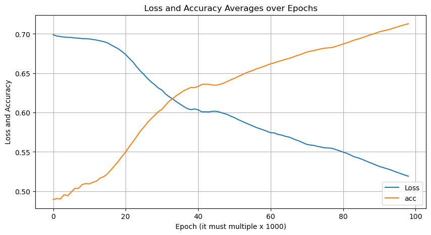

Epoch 99000/100000, Loss: 0.5191, acc : 0.7128917889718286

Test

마지막으로, 수열의 길이에 따른 정확도를 확인해볼 것이다.

from collections import defaultdict

length_total = defaultdict(int)
length_correct = defaultdict(int)

with torch.no_grad():
    for i in range(100000):
        if i % 5000 == 0:
            print(f"{i}번 test 진행")
        if i == (100000-1):
            print(f"{i}번 test 진행")
        x, target, sequence = generate_sequence()

        output, _ = model(x)
        output = output[-1:]

        length_total[len(sequence)] += 1
        if torch.argmax(output.squeeze()) == target.item():
            length_correct[len(sequence)] += 1

0번 test 진행
5000번 test 진행
10000번 test 진행
15000번 test 진행
20000번 test 진행
25000번 test 진행
30000번 test 진행
35000번 test 진행
40000번 test 진행
45000번 test 진행
50000번 test 진행
55000번 test 진행
60000번 test 진행
65000번 test 진행
70000번 test 진행
75000번 test 진행
80000번 test 진행
85000번 test 진행
90000번 test 진행
95000번 test 진행
99999번 test 진행

fig, ax = plt.subplots()
x, y = [], []
for i in range(2, 20, 2):
    x.append(i)
    y.append(length_correct[i] / length_total[i])
ax.plot(x, y);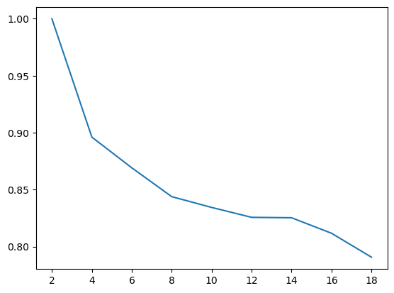

보다시피 수열의 길이가 늘어날수록 정확도가 떨어지는 양상을 확인할 수 있다.
이는 step이 길어짐에 따른 Gradient Vanishing 현상으로 인한 것으로 보인다. 이러한 배경으로 인해 LSTM이 탄생되게 된다.

'딥러닝' 카테고리의 다른 글

[Pytorch] Semantic Segmentation (1)	2024.10.18

현재글[Pytorch] RNN(Recurrent Neural Network)

Woohh 기록 보관소

주로 공부하며 기록하는 곳 입니다 :)

seq2seq, 바코드, 아스키코드, yolo, pytorch, 레지스터, 2진수, Segmentation, 디지털, NLP, bcd코드, 딥러닝, gray코드, 컴퓨터비전, 논리회로, CNN, U-Net, GAN, RNN, Ai,

Today :
Yesterday :

Woohh 기록 보관소